LSTM-Based Dynamic Pricing in Home RetailIt is no secret that machine learning methods have become widespread in various business areas: optimizing, improving and even creating new business processes. One important area is the question of setting the price, and here, with enough data, ML helps to do what was previously difficult to achieve — to reconstruct a multi-factorial demand curve from the data. Thanks to the restored demand curve, it became possible to build dynamic pricing systems that allow you to optimize the price depending on the goal of pricing — to increase revenue or profit. This article is a compilation of research case, in which it has been developed and tested the LSTM-ANN dynamic pricing model for one of the products of a home goods retailer. I want to note right away that in this article I will not disclose the name of the company in which the study was conducted (nevertheless, it is one of the companies from the list presented in the background), instead I will name it — Retailer. Background In the home goods retail market, there is a price leader — Leroy Merlin. The sales volumes of this network allow them to maintain a minimum price strategy for the entire product range, which leads to price pressure on other market players. Revenue and profit of the main retailers in St. Petersburg as of December 31, 2017:
In this regard, the Retailer uses a different approach to pricing: — the price is set at the level of the lowest of the competitors; — limit on the price below: purchase price + minimum markup, reflecting the approximate costs per unit of goods. This approach is a combination of the costly pricing method and focus on competitors’ prices. However, it is not perfect — it does not directly take into account consumer demand directly. Due to the fact that the dynamic pricing model takes into account many factors (demand, seasonality, promotions, competitor prices), and also allows you to impose restrictions on the proposed price (for example, from below — cost coverage), this system potentially gets rid of all one-sidedness and disadvantages of other pricing methods. Data For research, the company provided data from January 2015 to July 2017 (920 days / 131 weeks). This data included:
In addition to this data, I also added calendar dummy variables:
As well as weather variables:
By directly analyzing the daily sales of goods, I found that: Only about 30% of the products were sold all the time, all other products were either put on sale later than 2015 or removed from sale earlier than 2017, which led to a significant limitation in the choice of goods for research and price experiment. This also leads us to the fact that due to the constant change of products in the store line, it becomes difficult to create a complex per-item pricing system, however, there are some ways to get around this problem, which will be discussed later. Price recommendation system To build a price recommendation system for a product for the next period based on a model that predicts demand, I came up with the following scheme: 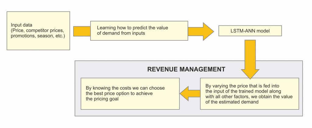 Feeding various prices as input to the trained model, we will receive sales estimation. Using such model we can optimize the price to achieve the desired result — to maximize the expected revenue or expected profit. It remains only to train a model that could predict sales well. What didn’t worked After selecting one of the products to research, I used XGBoost before going directly to the LSTM model. I did this in the hope that XGBoost will help me discard a lot of unnecessary factors (this happens automatically), and use the remaining ones for LSTM models. I used this approach consciously, because I wanted to get a strong and, at the same time, a simple justification for the choice of factors for the model, on the one hand, and on the other, to simplify the development. In addition, I received a ready-made, draft model, on which I could quickly test different ideas in the study. And after that, having reached the final understanding of what will work and what will not, make the final LSTM model. To understand the task of forecasting, I will give a graph of the daily sales of the first selected product: 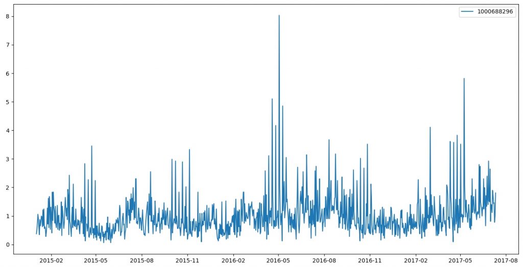 The entire sales time series on the chart was divided by the average sales for the period, to not reveal the real values, but to keep the view. In general, there is a lot of noise, while there are pronounced bursts — this is the conduct of promotions at the network level. Since this was my first experience building machine learning models, I had to spend quite a lot of time reading various articles and documentation in order for me to eventually get something. Initial list of factors that affects sales:
A total of 380 factors were obtained. (2.42 observations per factor). Thus, the problem of cutting off non-significant factors was indeed high, but XGBoost helped to cut the number of factors to 23 (40 observations per factor). The best result after hyperparameters greed search looks like this: 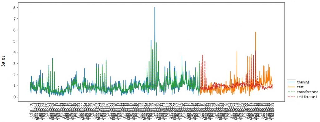 R^2-adj = 0.4 on the test set The data was divided into training and test samples without mixing (since this is a time series). As a metric, I used the R^2 indicator, adjusted deliberately, since it’s most common for regression tasks and easy to understand. The final results reduced my faith in success, because the result of R^2-adj 0.4 meant only that the prediction system would not be able to predict demand for the next day well enough, and the price recommendation would differ little from the random system. Additionally, I decided to check how effective the use of XGBoost would be for predicting daily sales for a group of goods (in pieces) and predicting the number of checks in the whole network. Sales by product group: 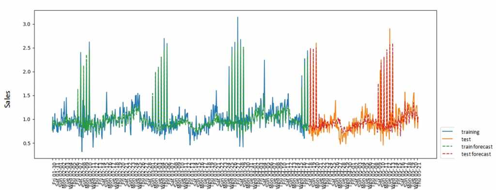 Checks: 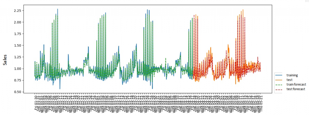 I think the reason that sales data for a particular product could not be predicted is clear from the graphs presented — noise. Individual sales of goods turned out to be too random, so the regression method was not effective. At the same time, by aggregating the data, we removed the influence of randomness and got good predictive capabilities. In order to finally convince myself that predicting demand one day ahead is a meaningless exercise, I used the SARIMAX model (the statsmodels package for python) for daily sales: 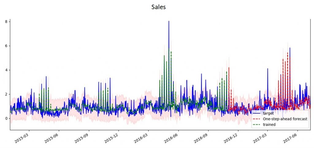 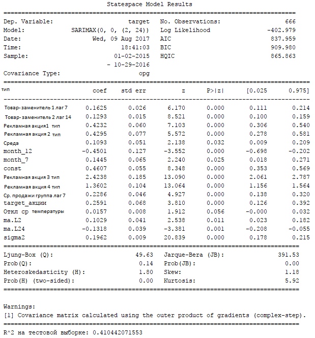 In fact, the results do not differ in any way from those obtained using XGBoost, which suggests that the use of a complex model in this case is not justified. At the same time, I also want to note that weather factors were not significant for either XGBoost or SARIMAX.
Building the final model The solution to improve the quality of the prediction was to aggregate the data to a weekly level. This made it possible to reduce the influence of random factors, however, it significantly reduced the number of observed data: if there were 920 daily data, then only 131 weekly data. Decreased greatly. In addition, my task was complicated by the fact that at that time, the company decided to change the product on which the experiment will be carried out to new product -primer CERESIT, so I had to develop the model from scratch. The product was changed to a product with a pronounced seasonality: 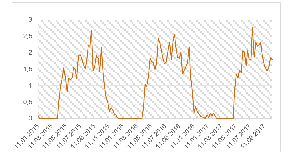 Due to the transition to weekly sales, a question arose: is it generally adequate to use the LSTM model on such a small amount of data? I decided to find out in practice and, first of all, to reduce the number of factors. I threw out all the factors that are calculated on the basis of sales lags (averages, RSI), weather factors (on the daily data, the weather did not play a role, and the conversion to the weekly level, all the more, lost any meaning). After that, I used XGBoost to cut off other unimportant factors. Subsequently, I additionally cut out a few more factors, based on the LSTM model, simply excluding the factors one by one, retraining the model and comparing the results. The final list of factors looks like this:
There are 15 factors in total (9 observations per factor). The final LSTM model was written using Keras, included 2 hidden layers (25 and 20 neurons, respectively), and an activator — a sigmoid. Final LSTM model code using Keras: model = Sequential() model.add(LSTM(25, return_sequences=True, input_shape=(1, trainX.shape[2]))) model.add(LSTM(20)) model.add(Dense(1, activation=’sigmoid’)) model.compile(loss=’mean_squared_error’, optimizer=’adam’) model.fit(trainX, trainY, epochs=40, batch_size=1, verbose=2) model.save(‘LSTM_W.h5’) Result: 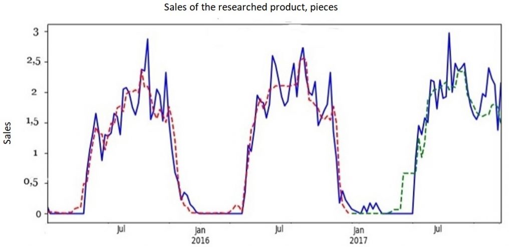
The quality of the prediction on the test sample looked quite convincing in terms of the metric, however, in my opinion, it still fell short of the ideal, because, despite the fairly accurate definition of the average sales level, spikes in individual weeks could deviate quite a lot from » average» level of sales, which gave a strong deviation of the sales forecast from reality on certain days (up to 50%). However, I have already used this model directly for the experiment in practice. It is also interesting to see what the reconstructed price demand curve looks like. To do this, I ran the model over a range of prices and, based on the predicted sales, built a demand curve: 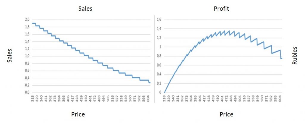 Experiment Each week, I have been provided sales data for the previous week in St. Petersburg, as well as prices from competitors. Based on this data, I performed price optimization to maximize the expected profit based on trained LSTM model, and this price was used in real world for the next week. This went on for 4 weeks (the period was agreed with the retailer). Profit maximization was carried out with restrictions: the minimum price was the purchase price + fix. surcharge, the maximum price was limited to the price of a Primer from the same manufacturer. The results of the experiment are presented in the tables below: Sales volume prediction:
Profit prediction:
In order to evaluate the impact of the new pricing system on sales, I compared sales for the same period, only for previous years. Summary results for 4 weeks:
As a result, we get a twofold picture: completely unrealistic forecasts in terms of sales, but, at the same time, purely positive results in terms of economic indicators (both in terms of profit and revenue). The explanation, in my opinion, is that in this case, the model, while incorrectly predicting the volume of sales, nevertheless, caught the right idea — the price elasticity for this product was below 1, which means that the price could be increased, not fearing for a drop in sales, which we saw (sales in pieces remained approximately at the same level as last year and the year before). But you should also not forget that 4 weeks is a short period and the experiment was conducted on only one product. In the long run, overpricing goods in a store usually leads to a drop in sales in the store as a whole. To confirm my guess on this, I decided to use XGBoost to check if consumers have a “memory” for prices for previous periods (if in the past it was more expensive “in general” than competitors, the consumer goes to competitors). Whether the average price level for the group for the last 1, 3 and 6 months will affect sales by product groups? 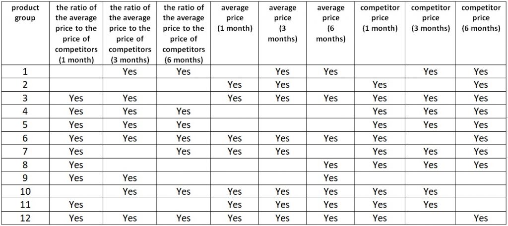 Indeed, the guess was confirmed: one way or another, the average price level for previous periods affects sales in the current period. This means that it is not enough to optimize the price in the current period for a single product — it is also necessary to take into account the general price level in the long term. Which, in general, leads to a situation where tactics (profit maximization now) contradict strategy (survival in the competition). This, however, is already better left to marketers. Given the results obtained and the experience in my opinion, the most optimal pricing system based on the sales forecast could look like this:
|

LSTM-Based Dynamic Pricing in Home Retail |
How Can We Help
We specialize on tailoring individual solutions for each company, emphasizing and fortifying your unique competitive advantage and corporate «DNA». We achieve this by seamlessly integrating leading business practices, concepts, and technologies. Our expertise encompasses a range of key areas:
17/09/2021